Vocal Tract Length Normalization (VTLN)
Calculate the Vocal Tract Length
Using Praat
After we installed the Pratt together with the VocalToolkit : https://www.praatvocaltoolkit.com/calculate-vocal-tract-length.html, we can just calculate the vocal tract length from the pratt easily.
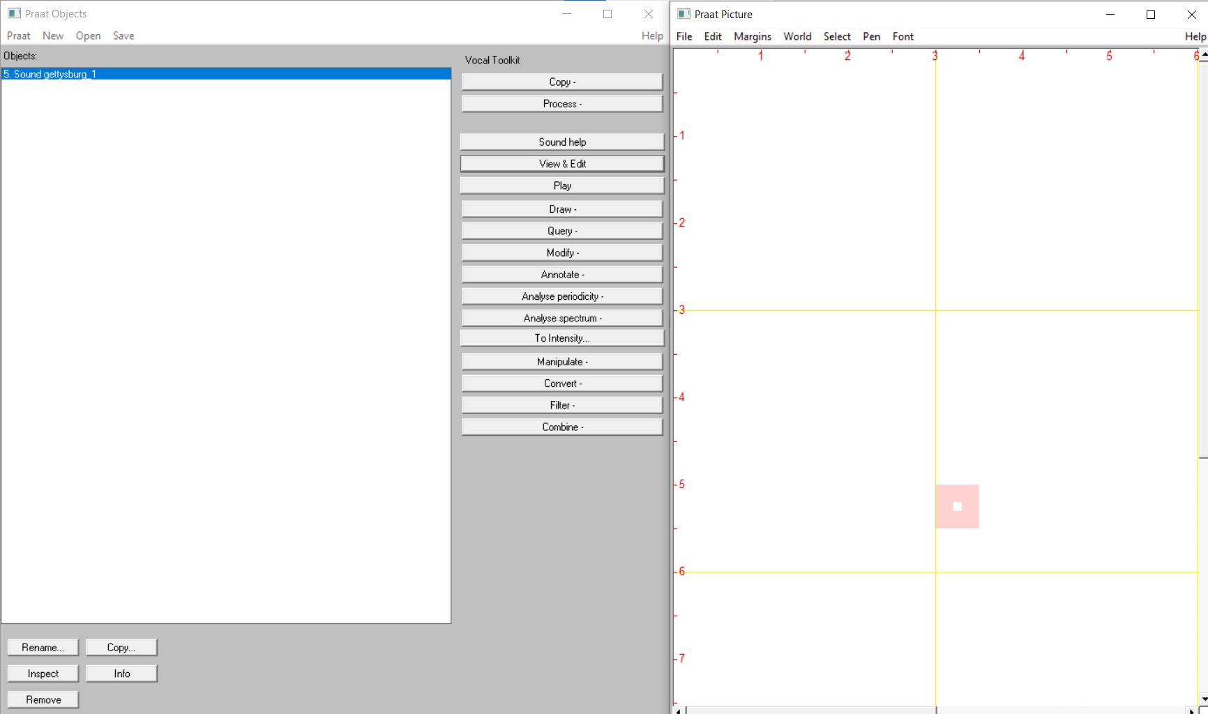
We can open that Praat the main panel, and hit the process buttom,
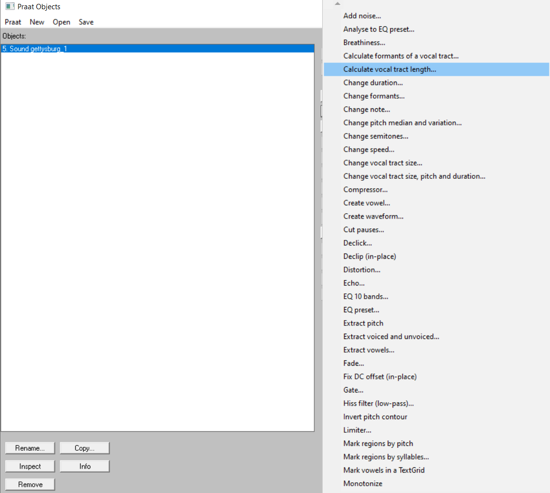
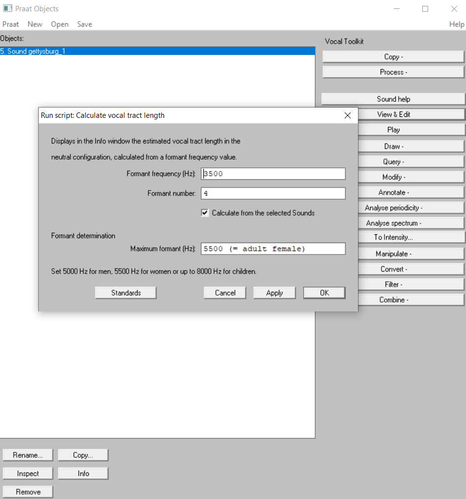
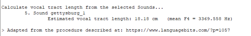
Here is the result, and the calculating formula was from: Johnson, Keith. Acoustic and Auditory Phonetics. 2nd ed. Malden, Mass: Blackwell Pub, 2003. p. 96.
$$
F_{n} = \frac{ (2n - 1)c}{4L}, c = 35,000\ cm/ sec
$$
In here, $$F_{4}$$ is 3369.558 Hz, and here can be the how it calculated:
$$
3369.558 \ Hz = \frac{(7)* 35,000\ cm/ sec}{4L} \
3369.558 \ \frac{1}{sec} = \frac{(7)* 35,000\ cm/ sec}{4L} \
\frac{3369.558}{sec} = \frac{(7)* 35,000\ cm/ sec}{4L} \
\frac{3369.558 * 4L}{sec} = (7)* 35,000\ cm/ sec \
3369.558 * 4L = (7)* 35,000\ cm \
L = \frac{(7)* 35,000\ cm}{3369.558 * 4} \
L = \frac{245000}{13478} \
L = 18.1777711827 \ cm
$$
Python Code Work
1 | |
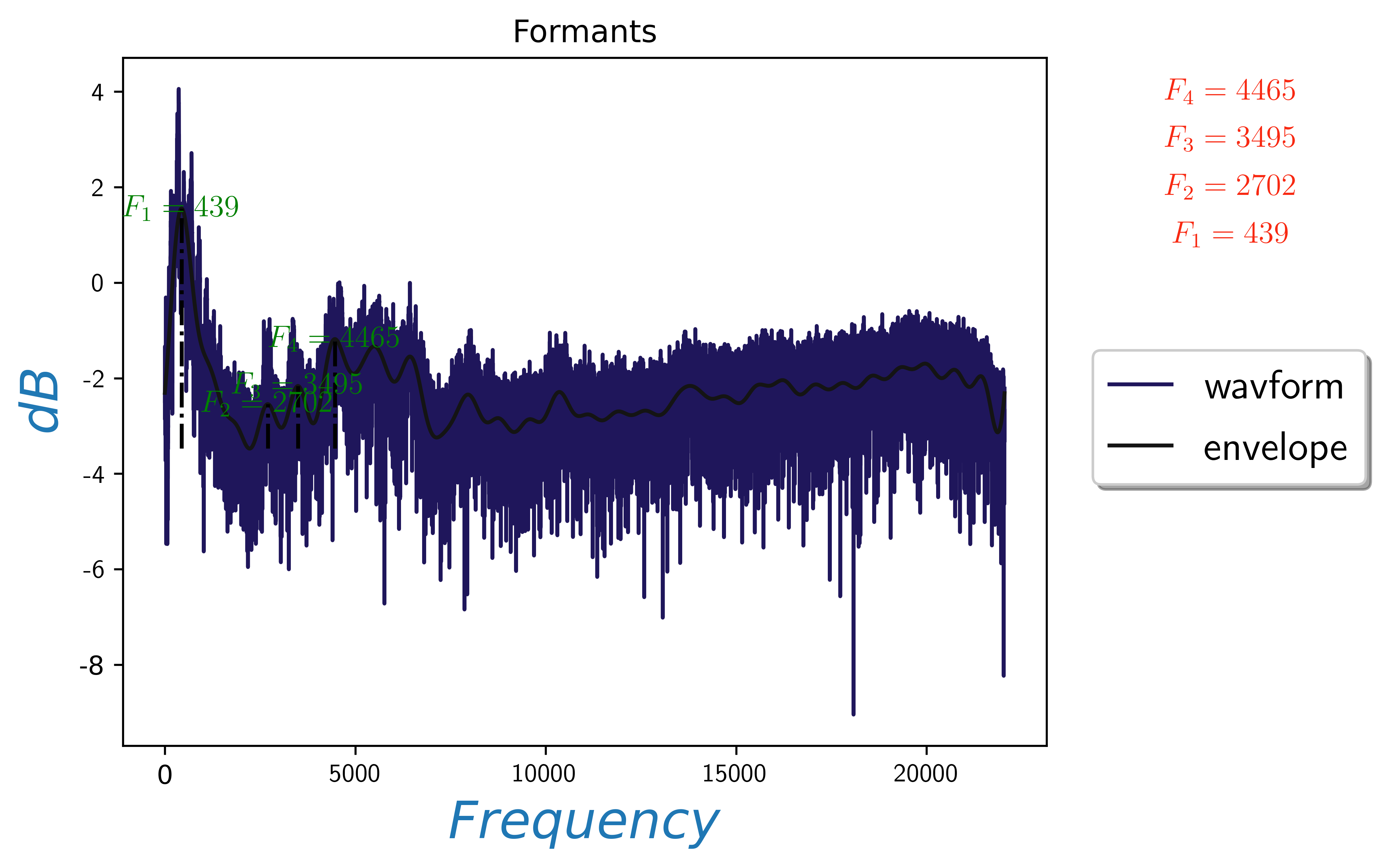
This will be the final visualization output:
Hamming Windowing
This is to add the hamming window:
1 | |
IFFT Work
This is the IFFT demo and save in the EPS file.
1 | |
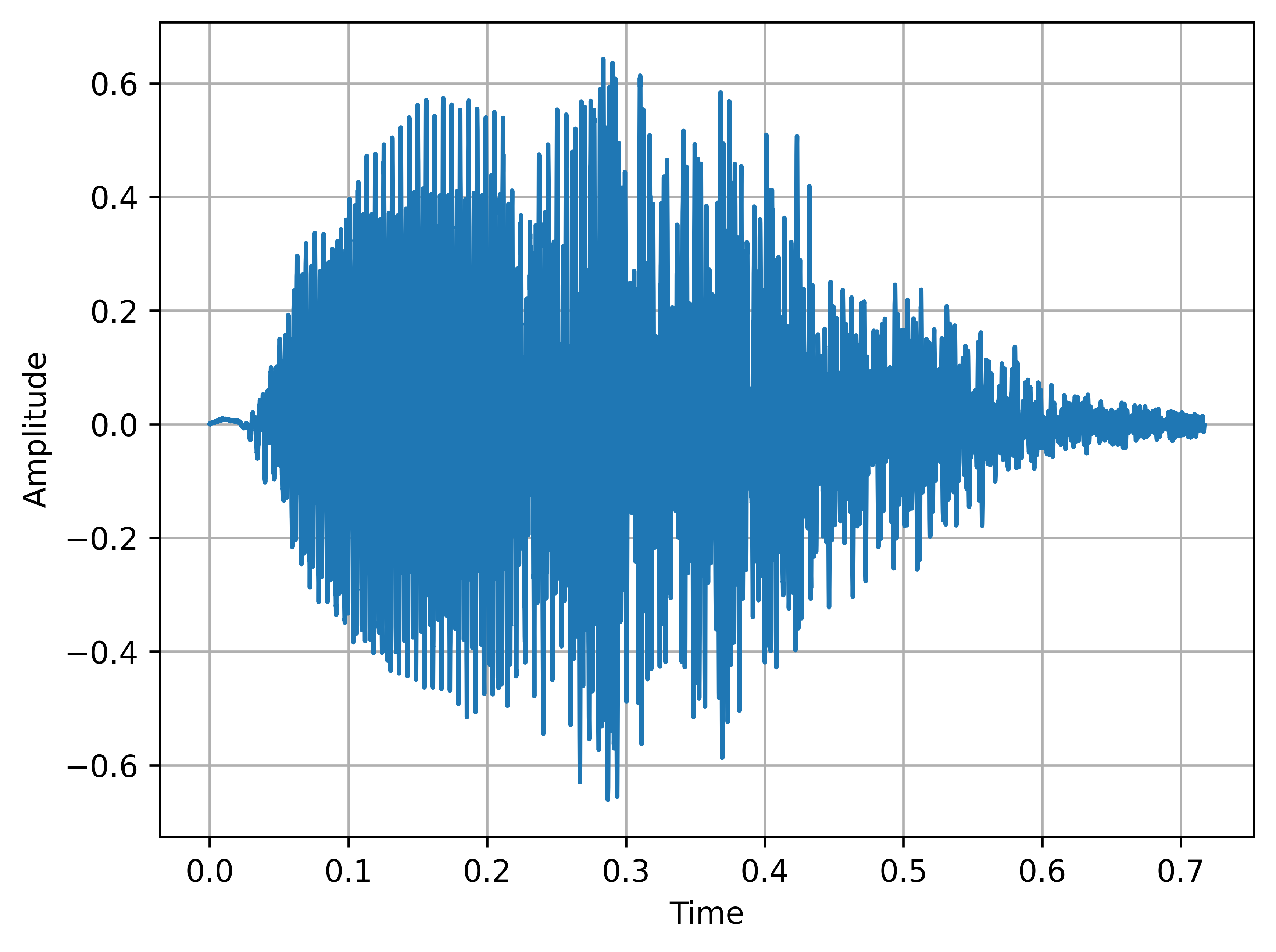
Cut Audio Chunks
1 | |
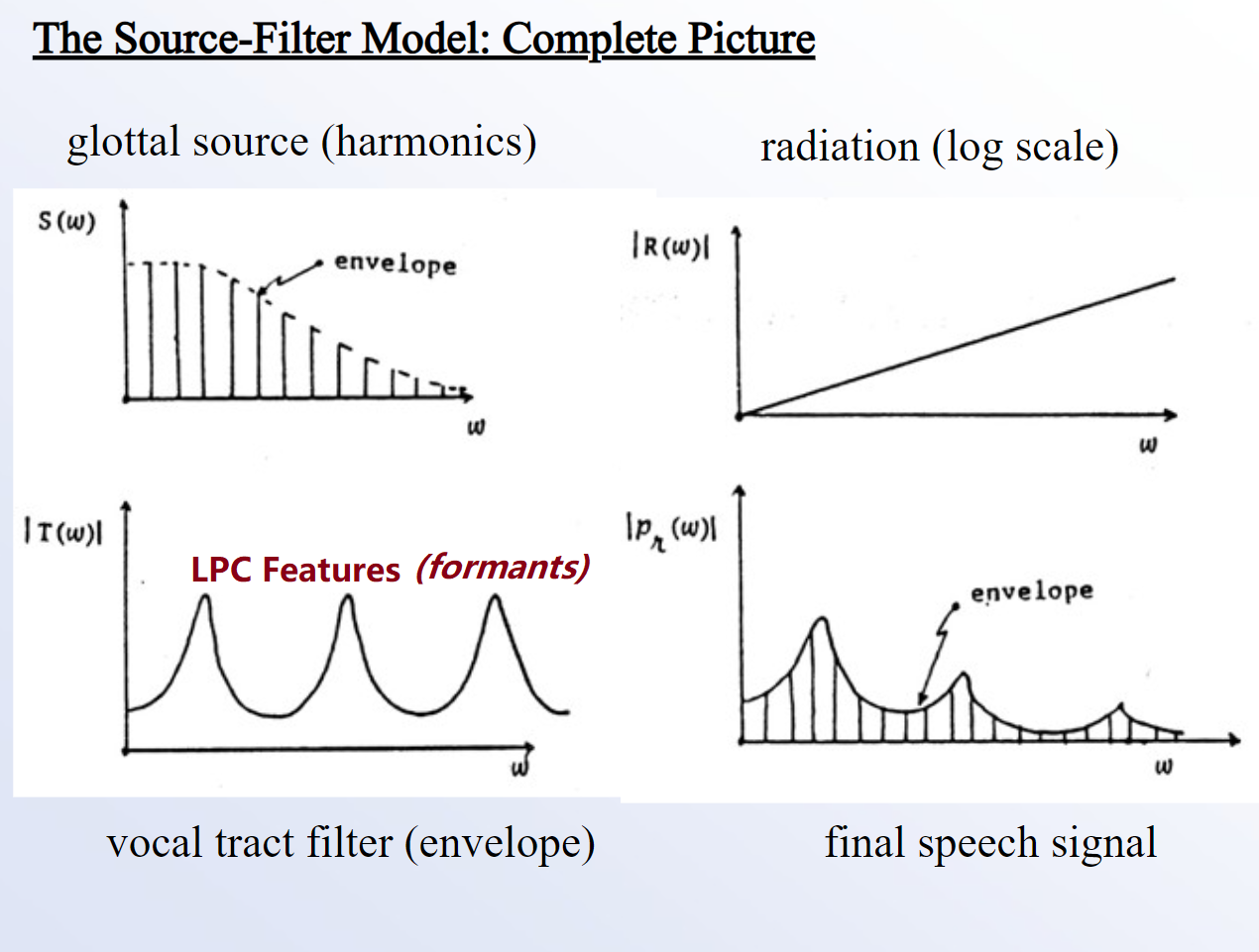
Source Filter Theory
https://slideplayer.com/slide/8271737/
https://www2.ims.uni-stuttgart.de/EGG/frmst1.htm